]")
]")

]")
]")
Ocean Biogeochemistry Lab
|
| |
Ocean Biogeochemistry Lab |
|
![]() The new SeaDAS is here... No more command line! What now... Below some help to get going again. This will work with Seadas 8 as well.
The new SeaDAS is here... No more command line! What now... Below some help to get going again. This will work with Seadas 8 as well.
SeaDAS 7 is based on BEAM (now SNAP) and can be freely installed. No more expensive IDL licenses! Plus it can analyze much more than just oceancolor satellite data. But it is completely different from Seadas 6, and there are still a lot of bugs and the GUI is not that stable.
On-line SeaDAS 7 help: SeaDAS Help index, the oceancolor forums and more on the SeaDAS website, incl. tutorials. Also the BEAM forum might be helpful. On the oceancolor website there is also a library of IDL routines, esp. the HDF functions might be useful (although some are for the older (hdf) format files, and not nc/hdf5).
Unfortunately there are no real practical HowTo pages on how to actually do stuff from the command line. I will try to provide some guidance below for mostly command line stuff with gpt and other programs like l3mapgen, so you can still use it with your IDL, R, Matlab, Python, shell, etc... scripts. For getting started with the GUI, check out the lab notes of the Remote Sensing course we teach here at Stanford. Update: There is now a very useful 'GPT Cookbook' on the seadas website with all kinds of expamples on how to use GPT.!
What is GPT - GPT = BEAM Graph Processing Tool. From the SeaDAS help: "This tool is used to execute BEAM raster data operators in batch-mode." So we can use it with scripts! Even IDL (or Matlab, R, whatever). The program name on Linux is gpt.sh, on a Mac it is gpt.command. Found in the bin subdirectory of the SeaDAS install. Example usage (in IDL you can use the 'spawn' command to execute this):
gpt.sh -e mosaic_sst.xml -Ssource=A20152132015243.L3m_MO_NSST_sst_4km.nc -t A20152132015243.L3m_MO_NSST_mapped.nc -f netCDF4-CF
where, input file is defined by source (A20152132015243.L3m_MO_NSST_sst_4km.nc), the output file after -t (A20152132015243.L3m_MO_NSST_mapped.nc), output format with -f (netCDF4-CF). The commands on what to do is included in the 'graph' file, in XML format (examples below). GPT has different functions, called 'operators', for example, Mosaic, Reproject, BandMaths. For help on these operators type: gpt.sh -h Mosaic for example.
GPT Mosaic Example - A simple example on how to reproject an image using the Mosaic operator with the following xml-file: mosaic_sst.xml. Usage identical to example above in 'What is GPT' section. Contents of XML file is very similar to the options in the GUI. Code explanation:
- Mosaic is the <operator>
- ${source} in <sources> is the input filename given on the command line
- sst is band to Mosaic
- I put in some conditions to only use the 'Best' and 'Good' pixels
- The GUI is a great help to format the XML file, esp. to code the projection parameters. In the 'Create Mosaic File' window select File -> Display Parameters, gives the XML code that goes in the parameters section of the XML file, incl. variables and conditions.
l3mapgen stereographic - Level 3 binned files (L3b) cannot be reprojected with Mosaic. You will have to use l3mapgen (which is part of the SeaDAS processing components). When using the GUI for l3mapgen, the drop-down list for projections seems very limited, and doesn't include stereographic for example. But, yes, you can still use other projections than listed. SeaDAS/BEAM is using proj.4 for projections. So instead of selecting a pre-defined projection in the GUI, you can just type over it with a proj.4 projection string. For example, if you used the following parameters with the 'old' SeaDAS stored in greenland_map_pfile.par, using the SeaDAS/IDL command line, as:
mapimg, bands=[1], map_pfile="greenland_map_pfile.par"
You can do it in the 'new' SeaDAS from the Unix shell command line as (with the projections parameters stored in l3mapgen_greenland.par):
l3mapgen ifile=A20152132015243.L3b_MO_CHL.nc ofile=A20152132015243.L3m_MO_CHL_mapped.nc par=l3mapgen_greenland.par
Or, using the GUI, you can paste the iproj.4 projection string +proj=stere +lat_0=72.5 +lon_0=-50 in the projection field. What is nice with l3mapgen, compared to mapimg, is that you can set the actual resolution in km. Not nice is that images projected with l3mapgen (still) don't contain geolocation info [a SeaDAS problem], so you are a bit limited with what you can do with it in SeaDAS. Also, stereographic projections over the dateline might give unexpected results [a BEAM problem].
Alternatively, you can still use the new format L3b with the old SeaDAS 6 after you convert them. L3b-files now come in netCDF4 format, while SeaDAS 6 can only deal with HDF4 L3b files. You can use the SeaDAS 7 version of l3bin to output to HDF4 with option oformat=1:
l3bin in=A20150012015008.L3b_8D_CHL.nc out=A20150012015008.L3b_8D_CHL.main oformat=1 noext=1
GPT Mosaic + Math Band Example - With gpt you can combine operators. For example, you can first project a band and then do some manipulations with Math Band on it in one go. In the example above after Mosaic'ing the sst file, all missing data were set to 0 instead of NaN, which is kind of silly since 0 can be a valid SST... With BandMaths (the gpt operator for Math Band) you can set it to NaN. This is done after Mosaic'ing, so, even 'valid' 0s will be set to NaN. Execution is similar as before, using mosaic_bandmath_sst.xml as the 'graph' file:
gpt.sh -e mosaic_bandmath_sst.xml -Ssource=A20152132015243.L3m_MO_NSST_sst_4km.nc -t A20152132015243.L3m_MO_NSST_mapped.nc -f netCDF4-CF
Notes on the code:
- A new node (with id bandMathNode) was added to the original file
- gpt Operator is BandMaths
- The source is not the input file but the result from the "mosaicNode"
- Expression syntax is the same as Math Band GUI (good for testing)
- A better way to set 0s to NaN and avoid mislabelling valid data is to use the sst_count band. Instead of using sst == 0 then NaN else sst use if sst_count == 0 then NaN else sst in the BandMaths operator.
In the GUI you can use MathBands with un-collated files as well (they have to be projected the same). If you have 3 files loaded you can use Math Bands code like: (($1.chlor_a > 0.0 ? $1.chlor_a : NaN) + ($2.chlor_a > 0.0 ? $2.chlor_a : NaN) +($3.chlor_a > 0.0 ? $3.chlor_a : NaN)) / 3.0, where $1, $2 and $3 refer to the 3 files. You can also do something similar from the command line. See for example myGraph.xml, run it as gpt myGraph.xml. See: this post on the Earthdata forum.
Passing parameters on command line - In the previous examples parameters were hard coded, like for example lat/lon boundaries. Which is fine in a lot of cases, but not when you are trying to output results from pixel value extraction for example. There is a way to pass parameters from the command line with the -P flag. From gpt.sh -h: -P<name>=<value> Defines a processing parameter, <name> is specific for the used operator or graph. In an XML graph, all occurrences of ${<name>} will be replaced with <value>.. So for example the latitude and longitude can be specified on the command line (rather than hardcoded in the XML file pixex.xml) as follows:
gpt.sh -e pixex.xml -Ssource=A20152132015243.L3m_MO_NSST_sst_4km.nc -Plat_in=32. -Plon_in=-120.
Notes on the code:
- Instead of hard-coding 32. in the <latitude> part of the XML file, we are using ${lat_in} instead, and is replace with 32. from the command line, using -Plat_in=32.
- It is easiest to create the code for the parameters section with the Pixel Extraction GUI and modify if necessary (see GPT Mosaic Example above).
To extract pixel information (including x and y locations) from multiple coordinates using PixEx is possible as well. Put the lat/lon in a tab-delimited file, with header line Name Lon Lat (example: coords.txt). You can use the above pixex.xml as well to reference the coordinatesFile. See gpt -h PixEx for more options.
infile=infile=/data1/gertvd/chla/mapped/MERGED/chukchi/MERGED.20230602.L3b_DAY_CHL_R2022.0_max30_L3m_NRT.nc
gpt PixEx -PcoordinatesFile=/home/gertvd/PixEx/coords.txt -PoutputDir=/home/gertvd/PixEx/out $infile
Using with IDL Executing shell commands like l3mapgen or gpt.sh can be done with the IDL procedure 'spawn', for example:
IDL> cmd = 'l3bin in=A20150012015008.L3b_8D_CHL.nc out=A20150012015008.L3b_8D_CHL.main oformat=1 noext=1'
IDL> spawn, cmd
With SeaDAS 6 it was also possible to run scripts directly from the command line (seadas -b program.scr). Here is an example to do something similar in IDL, with command line options.
First line of program l3b_proj.pro: pro l3b_proj, year=year, execute from command line as:
[albedo:~ 1043]$ idl -e "l3b_proj, year='2016'"
Reading netCDF4 files with IDL
IDL> nc_file = 'A20152132015243.L3m_MO_CHL_mapped.nc' ; mapped file generated with l3mapgen above
IDL> ncdf_list, nc_file, /var, /dim, /vatt ; will list variable/dimension info
IDL> var = 'chlor_a' ; found with above command
IDL> fileid = ncdf_open(nc_file)
IDL> varid = ncdf_varid(fileid, var)
IDL> ncdf_varget, fileid, varid, chlor_a ; put data in array chlor_a
IDL> ncdf_close,fileid
An even easier way:
IDL> var = 'chlor_a'
IDL> ncdf_get, nc_file, var, result
IDL> chl = result[var, 'value']; hash

IDL> ; help with hashes
IDL> print, result['chlor_a']
IDL> print, result['chlor_a','attributes']
IDL> .run
- if (result['chlor_a','attributes'].HasKey('add_offset')) then begin
-     chl_offset = result['chlor_a','attributes','add_offset']
- endif
- end
Level 3 binned files are a bit harder to open. The data is in a 'group' (from the command line check out the contents with: ncdump -h l3b_filename). It is easier to extract data with HDF5 routines. (You can also use 'l3bindump' to retrieve data):
IDL> l3b_file = 'A20152132015243.L3b_MO_CHL.nc'
IDL> file_id = H5F_OPEN(l3b_file)
IDL> ; retrieve fields in BinList and chlor_a
IDL> group='level-3_binned_data'
IDL> grp_id = h5g_open(file_id, group)
IDL> dataset = 'BinList'
IDL> dset_id = h5d_open(grp_id, dataset)
IDL> binlist_grp = h5d_read(dset_id)
IDL> h5d_close, dset_id
IDL> dataset = 'chlor_a'
IDL> dset_id = h5d_open(grp_id, dataset)
IDL> chlor_a_grp = h5d_read(dset_id)
IDL> ; calculate mean chlorophyll by dividing sum with weights
IDL> chlor_a_weights = binlist_grp.weights
IDL> chlor_a_sum = chlor_a_grp.sum
IDL> chlor_a = chlor_a_sum / chlor_a_weights  ; mean = sum/weights
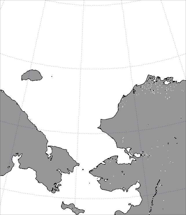
Creating Landmask + Grid Image
To create a landmask/coastline image plus gridlines in the same dimensions as your data is not very straightforward with the Export Image feature in the GUI. One way to do it is to load an image with the projection you want, make all data NaN, add landmask/coastline and gridlines. Then Export Image, under Source Boundaries check Data to retain the same dimensions. The result is a PNG file with a transparent background (see example). To make all data NaN in an image: right click on the band, select Properties. Under Valid pixel expression set the count to a high number. Example: chlor_a_count > 50. For best results, make the landmask and coastline in your 'final' color (eg. 150,150,150 [gray] for land and 0,0,0 [black] for coastline). It also helps with transparency to make gridlines black with grid line transparency set to 0.0.
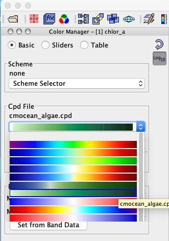
cmocean for SeaDAS
Kristen Thyng et al. created more user-friendly oceanographic color palettes. See her GitHub site. I converted the color palettes into SeaDAS cpd format. Find all palettes in this zip file or on my GitHub. Unzip the file and put the cpd files of interest in the ~/.seadas/beam-ui/auxdata/color-palettes directory (for SeaDAS 8 use: ~/.seadas8/auxdata/color_palettes). Restart SeaDAS and then they should be present, see screenshot.
Creating True Color Images
Look into BlueMarble. From an Announcement email by NASA/DRL:
You may access BlueMarble v1.8 at the Direct Readout Web Portal:
http://directreadout.sci.gsfc.nasa.gov/?id=software
For your convenience, the BlueMarble v1.8 User Guide is located at:
https://directreadout.sci.gsfc.nasa.gov/links/rsd_eosdb/PDF/BLUEMARBLE_1.8_SPA_1.8.pdf
Facebook: https://www.facebook.com/directreadout/
More to come...
Page by: Gert van Dijken