![[Table iceberg at sunrise, off Neumayer Station, Antarctica]](/images/random/thumb_iceberg_sunset2.jpg)
![[Collectors of a fancy sediment trap to be deployed in the Amundsen Polynya (ASPIRE/NBP1005)]](/images/random/thumb_DSC0325.jpg)
![[Arrigo-Icescape team, Zach, Matt, Gert, Kevin, Kate, Molly and Haley (Icescape/HLY1001)]](/images/random/thumb_DSCN1899.jpg)
![[Pine Island Glacier (January, 2009)]](/images/random/thumb_DSCN6590.jpg)
![[ocean.stanford.edu itself]](/images/random/thumb_oceanin.jpg)
![[Table iceberg at sunrise, off Neumayer Station, Antarctica]](/images/random/thumb_iceberg_sunset2.jpg) ![[Collectors of a fancy sediment trap to be deployed in the Amundsen Polynya (ASPIRE/NBP1005)]](/images/random/thumb_DSC0325.jpg) ![[Arrigo-Icescape team, Zach, Matt, Gert, Kevin, Kate, Molly and Haley (Icescape/HLY1001)]](/images/random/thumb_DSCN1899.jpg) ![[Pine Island Glacier (January, 2009)]](/images/random/thumb_DSCN6590.jpg) ![[ocean.stanford.edu itself]](/images/random/thumb_oceanin.jpg)
| |
Ocean Biogeochemistry Lab |
|
The goal of this lab is to learn how to order and process images. You will use Section 1 (Ordering Data) as a reference later for your project.
For today, download one ocean color image and move on to Section 2 (Processing to Level 2).
Contents:
1. Ordering Satellite Data
2. Processing to Level 2
Ordering SeaWiFS imagery (1997-present,S***)
For this class purpose, choose only a day's worth of images. After clicking
'find swath', a new page appears , with many scenes. Enter your password
on the top left menu 'SeaWiFS user login'. You can download any one scene
directly by subsequent clicking on the file name. If ordering more than one
scenes click 'order data' (top right) , Enter your valid email id. Click next
to *Do Not* extract my order for me. Click on desired products below
Level 1 / Level 2 and ancilliary products. Click Review order and Submit
order in next page.
After you have clicked away confirming your order, you will get a confirmation by e-mail from the GSFC. Reply to that (without writing anything in it, see instructions). A couple of mins/hours later (depending on the volume of data requested), or sometimes next day, you will get a 'Data Ready' e-mail with instructions where to ftp the data from. Download your data within 3 days, otherwise they might be deleted from the ftp-site. To FTP follow these instructions. Be sure to use the binary mode. You will likely want to FTP from your "documents" class folder, so that this is where the files download to.
Pathfinder/AVHRR: Download from NODC-NOAA website, select Available Data. Normally you would use '1. Direct FTP Access'
MODIS:
From the oceancolor.gsfc.nasa.gov website, the same as Chlorophyll.
Level 1 to Level 2 image processing
Level 1 files contain the radiance counts at each channel received by the
SeaWiFS sensor. To translate these to normalized water leaving radiance,
chlorophyll, etc. we have to process the files to Level 2 by applying atmospheric
corrections and bio-optical algorithms. The SeaDAS function to do this is
called: 'l2gen'. This program can generate a total of 176 (!) different products. See also Overview of SeaWiFS Data Processing and Distribution on the OceanColor website. There is a similar page for MODIS-Aqua.

|
| - What's in a SeaWiFS L1A file |
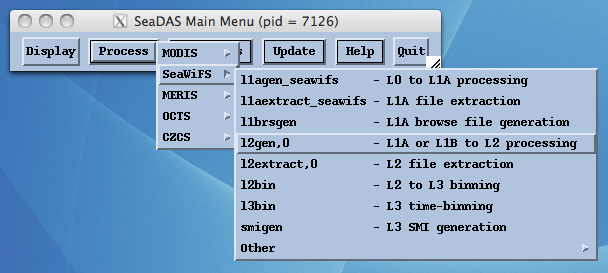
Select from the SeaDAS Main Menu: Process -> SeaWiFS -> l2gen,0 - L1A or L1B to L2 processing. Select the L1A input file in the 'SeaDAS SeaWiFS L2 File Generating Program' window -- the L1A input file that you moved to your personal directory. SeaDAS will automatically suggest the Level 2 output file name (first part of L1A file + L2 extension). Add something to this name that allows you to identify it as your own. SeaDAS will also automatically start checking if the needed ancillary files are present, like meteorological and ozone data. If they are not present SeaDAS will download them for you. Then for your output file (L2 output file 1) click on 'Select L2 Products' where you can make your choice of the 176 different products (see l2gen Output File 1 L2 Products Selection Widget). Take a look at these different products and see how many you recognize. You can choose as many products as you want, but each processing takes time. One L2 output file can contain more then one product (similar to the 8 bands stored in the L1A-file). However, you can also spread out some specific dataproducts over different L2-output files.
|
| - l2gen,0 Menu Option |
You can also do some subsampling of your image under the 'Subset/Subsample' tab in the SeaDAS SeaWiFS L2 Generation Program window. L1->L2 processing is very cpu intensive and can take quite some time. Therefore it is advised to select only the specific region on the image you are interested in for processing. This can be done by selecting the pixel and line range on the image or using lat/lon coordinates. Because we have a large class doing many computations, choose pixel and line subsampling interval of 4, to speed things up.

|
| - SeaWiFS L2 File Generation Program Window |
With Ancilliary files and processing options, you can manipulate the way msl12 (the SeaDAS software code that converts radiance to ocean products) will calculate the L2 products. Normally you leave them as is. By default SeaDAS will not try to use near real-time data which will be downloaded automatically. You can also opt for climatological data. If you want to manipulate the processing, click on the Processing Options tab. You can also change flag thresholds.
When you are ready to do the L2 processing, click on either 'Run' or 'Run(BG)'. The difference is that with 'Run(BG)' the process will run in the background and you can still do other things in SeaDAS. With 'Run' you have to wait until it is done before you can do anything else. If you have a list of files to process running it in the background is advised. After the run completes, find your L2 file using a new Terminal window. Now try loading it into SeaDAS and adding a colorbar. Do you recognize where this image is from? After you finish, be sure to compress your L2 file.
Processing MODIS-Aqua data requires 2 extra steps. From the OceanColor website you can get L1A_LAC data containing uncalibrated radiances at 19 bands (more info). We have provided a MODIS L1A_LAC file for you in the 'MODIS' folder of the Icy EESS141 home directory. Copy this file to your personal directory.

|
| - What's in a MODIS L1A_LAC file |
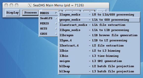
Unlike SeaWiFS, geolocation data (latitude/longitude info) is not included in the L1A file and has to be generated first. From the SeaDAS Main Menu, select: Process -> MODIS -> geogen_modis - L1A to GEO processing. Select your MODIS L1A input file. The output GEO file name is automatically generated. Click on Run to start the process.
|
| - Geolocate Menu Option |

|
| - MODIS Geolocate File Generation Program Window |
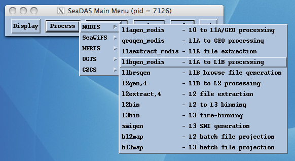
Now we are ready to create a L1B file which will contain calibrated radiances. From the SeaDAS Main Menu, select: Process -> MODIS -> l1bgen_modis - L1A to L1B processing. Select your Input L1A file.
|
| - l1bgen_modis Menu Option |
|
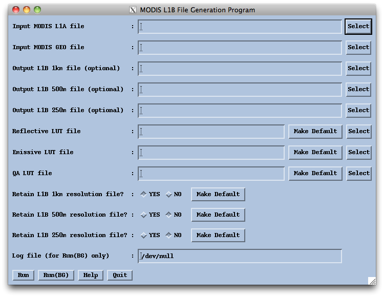
| - MODIS L1B File Generation Program Window |
If the file names are the same before the extension, it will automatically pick the geolocation file (GEO file) created in the previous step. If not, select the GEO file. Usually you only want to retain the LAC (1km) file. You can remove the other products by erasing the names with the HKM and QKM extensions. Click on Run. After it has finished you can select Display to see what Products have been generated.

|
| - What's in a MODIS L1B_LAC file |
|
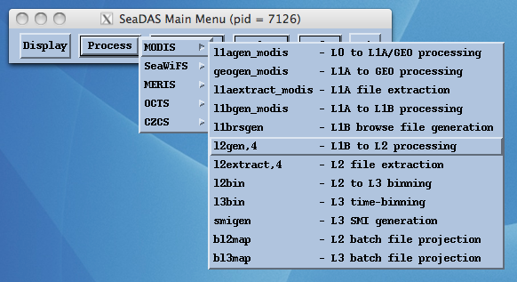
| - MODIS l2gen,4 Menu Option |
|
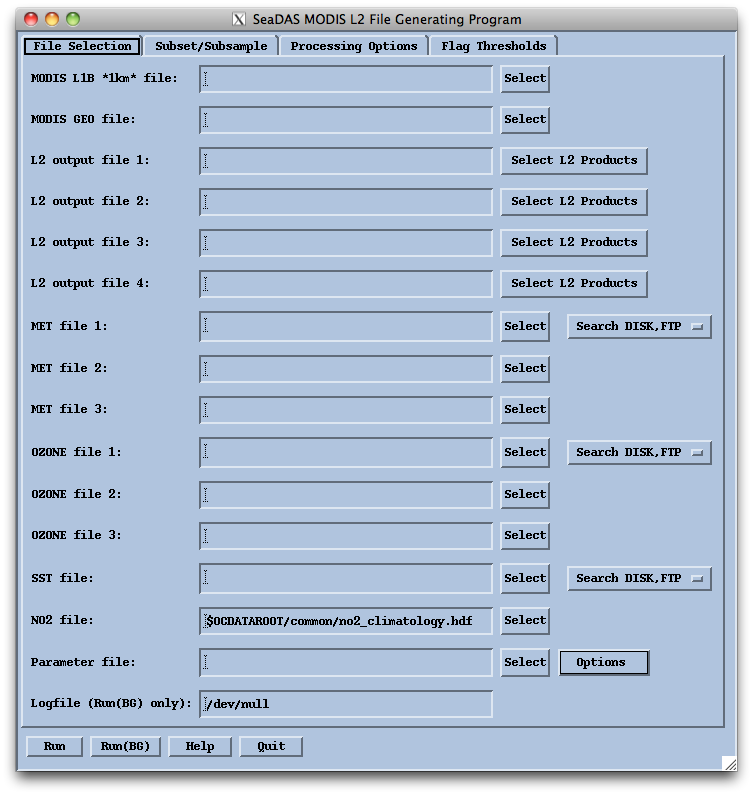
| - MODIS L2 File Generating Program Window |