]")
]")
]")
]")

Ocean Biogeochemistry Lab
|
| |
Ocean Biogeochemistry Lab |
|
During this course we will use SeaDAS (SeaWiFS Data Analysis System) extensively. Although it has been specifically developed for analyzing SeaWiFS data, other satellite data can be manipulated with this software package as well. SeaDAS has many, many features and it might be overwhelming at first. Luckily, there is a detailed help section on the different programs as well as a tutorial available on the SeaDAS website. The program can be run in two modes: interactive and command mode. We use the interactive mode with widgets/menus/etc.
In this lab we will load AVHRR SST satellite data into SeaDAS and then use some of the most commonly used functions in SeaDAS.
- See lab 2 notes on how to log into Mac rather than Windows and open a Terminal window.
Login to Icy (our server next door) using the command ssh -Y eess141@icy.stanford.edu. We will provide you the password. When you login, you'll be at the home directory.
- We have a couple of AVHRR files for you. To use them, navigate to the folder '/home/eess141/AVHRR'. Notice the way these files are named -- they are from both from 1997, one from July and one from December. Later, you'll be downloading and storing your own data on Icy.
- Start Seadas:
> seadas -em
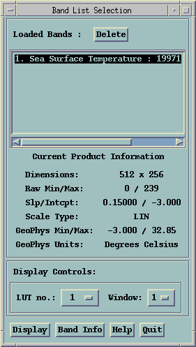
- Load the AVHRR images into SeaDAS. From the SeaDAS Main Menu, -> 'Display'. Note that at the top of the window, it shows you the current path, in this case, the one you started SeaDAS from. Choose one of the .hdf files and click ok. Click the box next to 'Sea Surface Temperature' and click 'Load'. Now load the other AVHRR image.
- Click 'display' on the Band List Selection to view one of the images. Briefly discuss some of the features with a neighbor. Do the east or west sides of ocean basins tend to be warmer? Why?
(Note: Minimizing 'Band List Selection' window minimizes all the other display windows. Maximize it again to get them back).
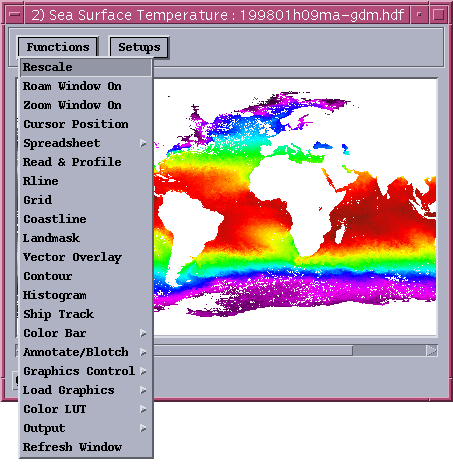
- Experiment with some of the different display functions in SeaDAS, like
In this lab we use some of the
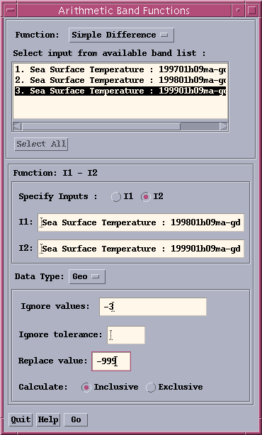
Arithmetic Band Functions:
[ Utilities-> Data Manipulation -> Simple Arithmetic]
With this function you will be able to calculate
- the difference between two scenes/images
- the average of two or more scenes and
- do a general summation of two or more scenes at each pixel.
More detailed information is available at this SeaDAS help section
Simple Difference:
We can use this for example to view the temperature difference between the months of December and July. This function will calculate the difference between
the two input bands, (I1 - I2) and creates a new band as a result (listed
as the last band in the 'Band List Selection' window).
- Select the two input bands (I1 and I2). For I2, click on bubble next
to I2 (next to 'Specify Inputs') and select from available band list (see figure).
- Select the the Data Type (raw or geo, normally you will use 'geo').
Other settings include 'Exclusion method', 'ignore tolerance', 'replace value' and 'inclusive' or 'exclusive' (see figure).
- About 'ignore value':
All points on an image have a specific value, even Land or Missing Data.
You don't want to include these data points when subtracting the two bands.
In the AVHRR images land and missing data are flagged with the value '-3'.
So if you would subtract the two bands you will get the value '0' at that
pixel. This would be the same value as at pixels where the temperature would
be the same for both input bands. To avoid this, we exclude all pixels with the value '-3'.
- Exclusion Method: a. Min./Max. This allows you look only at data from a range of minimum and maximum values, but is not what we want to use for this lab. b. Ignore/Tolerance. Select Ignore/Tolerance, which will tell SeaDAS to ignore all pixels with value '-3' (which is the default missing value in SST data) and giveb the option to replace them with another value. If you ignore -3 without replacing them with another value, then the missing and land pixels will be -3 in the resulting band. This might not really be the result you want. For example, there could be locations where the difference is really 3 degrees. These would be indistinguisable from land and/or missing data. This can be solved by replacing the -3 pixels in the input bands with a value which most probably will be out of range for 'good' data. So if you enter for replace value -999 you will get a new pixel value for land and missing data (instead of -3 it will be -999).
- 'inclusive' or 'exclusive' ?
You can have SeaDAS calculate the difference in inclusive or exclusive mode.
Inclusive mode means that it will calculate the difference only at pixels
where both the input bands have a valid (non-ignore) data point. For exclusive
only one of the bands has to have a non-ignore value. When you calculate
the difference between two input bands you would normally want to use inclusive
mode. Otherwise if you have a location where say the temperature is 28 degrees
for one input band, but the value at that location on the other input band
is missing (-3), SeaDAS will ignore the -3 and use as the difference 28 minus
nothing equals 28. Indeed, not the result you intended.
Example: Simple Difference:
                  Image1    Image2    Result I1-I2
      inclusive:    28        -3          -999
      exclusive:    28        -3           28
assuming: ignore value: -3; replace value: -999- Before making the calculation, think: where do you expect to observe the greatest SST differences between December and July? Will they be positive or negative?
Simple Mean:
[ Arithmetic Band Functions -> Function: Simple mean ]
- Choose Bands from list, as well as other fields as described for Simple
Difference.
- But, when you want to make a composite of different days or satellite scenes
by calculating an average you usually want to use the exclusive mode.
For example, SeaWiFS rotates around the earth a number of times per day. So
you can have 4 or 5 scenes on one specific day of the same location. When
you make a daily composite by taking the average of all these scenes you might
be able to get rid of most of the clouds. Since clouds move around they will
normally be at a different spot on each of your scenes. So during one of
the satellite overpasses the sensor might be able to collect some good data.
When you use exclusive mode it will use this data point for the calculation
of your daily composite. For example suppose you have 4 scenes available
of a day and you want to make a daily composite. If at a specific latitude
and longitude during three of the four overpasses the ocean is masked by
clouds, using exclusive mode will be able to still give a valid data point
for that specific location, thanks to the 4th overpass. If you would have
used the inclusive mode, because at least one of the scenes has a bad data
value, the data point would have been ignored.
Example: Simple Mean:- click on Go!
Image1 Image2 Image3 Result (I1+I2+I3)/3
inclusive: 28 -3 26 -999
exclusive: 28 -3 26 27
assuming: ignore value: -3; replace value: -999
Multiple Band Data Display
[ Seadas Main Menu -> Utilities -> Data visualization -> Multiple Product Data Display -> Geo Data view ]
This gives various information like Lat/Lon, geo/raw data at pixels pointed by mouse arrow on any displayed band. With different bands displayed it is a convenient way to find the data values at a specific point in each image.
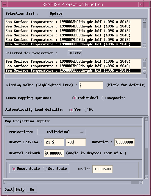
Projection
[ Utilities -> Data Manipulation -> Map Projection ]
With the Seadisp projection function you
can basically do two things. First you can map your image using a different
projection (e.g. cylindrical, mercator, stereographic, etc.). The AVHRR data
we downloaded are already projected on an 'equal-angle' grid. Not all satellite
data you will use will have been projected, i.e. the resolution may not be
the same for each pixel in the scene.
Second, you can use the projection function for is 'zooming'
in on the image. By using specific latitude/longitude pairs you can generate
new bands with only your area of interest. For help see this and/or this SeaDAS Help section.
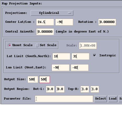
Important inputs (see figure):
Projections: select the type of projection. For example Cylindrical,
Mercator, ... Some projections are better for higher latitudes then others.
Center Lat/Lon: this is usually the latitude and longitude of the
center of your box you specify below. More info: SeaDAS Help.
Lat Limit (South, North): minimum and maximum latitude of your area
of interest. For southern hemisphere use negative degrees.
Lon Limit (West, East): see above. For degrees West use negative degrees.
Isotropic: Usually you check this option so that the newly projected
image will not be stretched in the latitude or longitude direction to fit
the output size you select below. So when you check isotropic the scale will
be the same in both the x and y direction. Try it to better understand it!
Output Size: Size of the display window of the mapped band. If you
make it too small you can lose resolution. You might have to experiment with
this option a little bit.
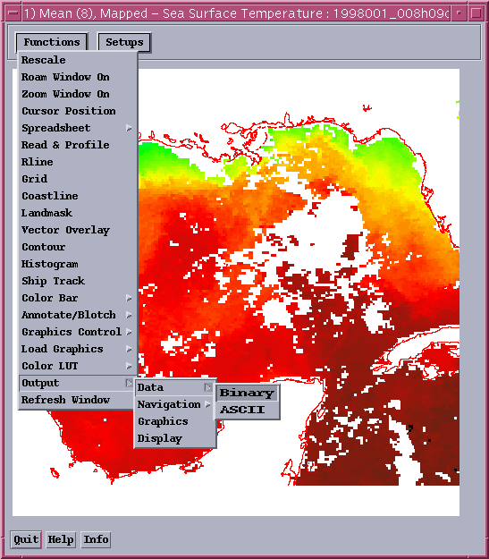
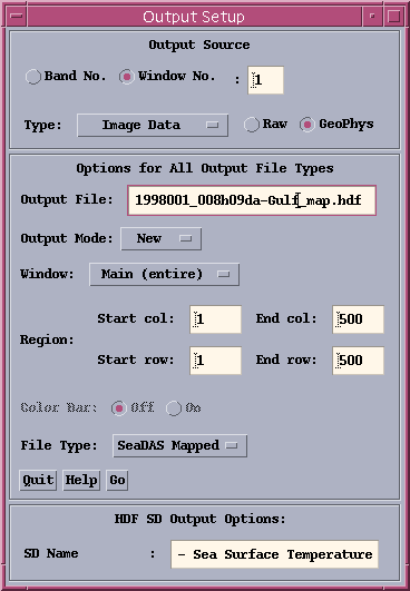
Output Data
Often you want to save one of the newly generated bands to a file so you can reuse it in another SeaDAS session. To do this select from the image window you want to save, Functions -> Output -> Data -> Binary. If you select as file type 'SeaDAS Mapped' for the projected bands it will be easy to reload them into SeaDAS (see figure). If you save it as 'HDF SD' you will lose the navigation (latitude/longitude) info. The type of data you want to save is 'Image Data', 'GeoPhys'. Rename the 'Output File' so that you can identify it as your own. It will automatically save to the folder from which you opened SeaDAS. Try opening a new terminal window, logging into Icy, and moving the file to your own folder that you already created. To double check if the data is really saved, load the newly saved data file using 'Display' as type 'SeaDAS Mapped'. Try to throw a grid or coastline on it. If that works then the navigation info has been saved with the geophysical data.
Lab over?
- Exit from Seadas: by clicking quit on the Seadas Main menu.